ACE : Age Calculation Engine

Here we show how to include user-generated modules into ACE.  As an example, we introduce Stone (2000) scaling.

Stone (2000) scaling resembles Lal (1991) scaling, so we start with the existing Lal algorithm and copy it.  Existing ACE modules are located in ACE/src/GUI/ACE/Components.  In this directory is a file called ‘LalScalingFunctions.py’.  Let’s duplicate it and rename the new file as ‘StoneScalingFunctions.py’.  Now open a text editor and look at this file.  Here is the header:

The first line is LalScalingFunctions.py and should be renamed to StoneScalingFunctions.py

The rest of the header text is comments (between “”” and “””), including the doi for the original Lal scaling.  Be sure to update this information when new science is added. The next part of the program introduces the Lal data (from Table 2 of Lal 1991) into the subroutine:

The first line class LalScalingFunctions should be renamed to StoneScalingFunctions, and again on the third line.

The term geolat refers to latitude, the term a1 to the polynomial coefficient a1 in Table 2 etc etc.  After these definitions there are four functions:

• self.setScalingFunctionSP(s),
• self.setScalingFunctionTH(s),
• self.setScalingFunctionMU(s), and
• self.setScalingFunctionMUfast(s).

The function take each sample (s) and return scaling functions for spallation (SP), low energy neutrons (TH), and slow (MU) and fast (MUfast) muons.  Note that the Lal 1991 pulication has no low energy or muon scaling, but it is included here for consistency with the scalings which do. Below is the code for spallation:

This function finds the latitude of the sample (defined in the code as s[“paleomagnetic latitude”], the attribute “paleomagnetic latitude” of the sample “s”) and interpolates the coefficients a1, a2, a3 and a4 to that paleomagnetic latitude, calling the interpolated coefficents a1_interp, a2_interp, a3_interp and a4_interp. Note that often for Lal scaling the current latitude of the sample is often used.  We choose to invoke paleomagnetic latitude as that is used by Lal.  As a consequence, the Lal scaling is not time invariant if a time varying geomagnetic latitude reconstruction is chosen. If time invariant Lal scaling is required, “present day” should be selected for geomagnetic latitude during the experiment design phase described in the previous online help section.

The local spallation production rate is then Equation 1 of Lal (1991).  We define it in the code as local_prod.

Then the scaling factor will be the local production rate divided by the production rate at high latitude and sea level.  In this case elev = 0, so Lal’s polynomial collapses to a1 at 90 degrees, which is a1[7].  Something to be careful about in Python is that in a list (lets call the list a1), the first entry is a1[0], not a1[1].  So even though a1 above have 8 entries, the last entry is a1[7].

Now we have a spallation scaling factor called s[“S_sp”] which can be passed to any other routine in ACE.  As an example, ACE outputs a variable called ‘scaling spallation’ which adds up s[“S_sp”] at each time step and then divides by the number of time steps to calculate the time averaged spallation scaling factor.

At this point we know just about everything we need to to make a Stone scaling module.  The muon scaling factors in this file are already set to those of Stone (Equation 3), and the low energy scaling factors are the same as for spallation.  Therefore the spallation scaling factors are all that require to be changed.  Let’s start with the polynomial coefficients.  From Stone Table 1 we can update the coefficients to:

Noting that we have renamed a1 to a, a2 to b, etc for consistency with the original equations in Stone (2000).  Instead of elevation, Stone uses atmospheric pressure (hPa, equivalent to mb) to calculate scaling.  Therefore we need to import pressure here:

Where the factor of 1.01959 is used to convert from g/cm2 to mb.  We repeat this line for pressure in the spallation scaling section.  When this is done we can calculate scaling using Stone (2000):

Note the use of the backslash to indicate line continuation equation.  In addition the high latitude, sea level production rate is no longer a constant, so we need to explicitly calculate it:

It is the same equation as before, but we use high latitude, sea level values.  The spallation scaling factor is just the ratio of these:

Done!  Well, almost.  We need to tell ACE what kind of option this new module is.  At the moment these are hardwired into the code, but in the future there should be a GUI for this.  In your ‘repo’ (repository) directory there is a file in the directory ‘factors’ called ‘geographicScaling.txt’.  Open it in a text editor:

This file lists the different types of geographic scaling that ACE has.  A lot of scaling functions use cutoff rigidity and there are different ways of calculating cutoff rigidity.  This file lists which cutoff rigidities should be used with which scaling functions.  For example the Desilets and Zreda (2003) scaling functions use cutoff rigidity calculated in the Python file ‘CutoffRigidity’.  The Lifton et al. (2005) scaling functions use the module ‘LiftonCutoffRigidity’.  The dating and calibration algorithms always have a placeholder for cutoff rigidity, but as  Stone scaling does not use cutoff rigidity it doesn’t matter what we specify here.  So we can add the following line to this file:

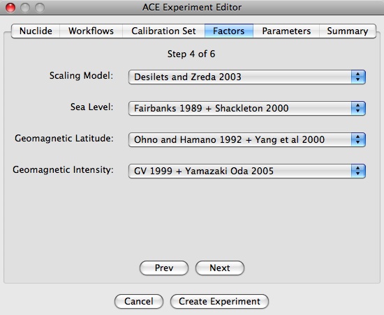
That is, we specify a new scaling in ACE which calls ‘StoneScalingFunctions.py’ and is labelled Stone (2000).  Let’s open the experiment browser in ACE and make a new experiment which uses it:

And see the results:

So using Stone scaling in a time-stepping formulation on ³He yields a HLSL production rate of 134 ± 7 atoms/g/yr.

This is a fairly simple example of module additions to ACE, but it should be noted here that changes are automatic in the sense that if Stone scaling is used in an experiment, it will be used both in the calibration and dating routines with appropriate production rates.  However if you want to make more fundamental changes to ACE, please email us.

The routine used to calculate Stone scaling is available for download: StoneScalingFunctions.py.